Main MCMC fit function

This function is the main MCMC function to fit a 2D Bezier spline to the limit set boundary of bivariate data in exponential margins

Usage

fit_mcmc_bezier(
  N,
  r,
  w,
  r_0,
  priors = list(p0y_mean = 0, p0y_sd = 1, p1x_mean = 0, p1x_sd = 1, p1y_mean = 0, p1y_sd
    = 1, p2x_mean = 0, p2x_sd = 1, p3_mean = 0, p3_sd = 1, p4y_mean = 0, p4y_sd = 1,
    p5x_mean = 0, p5x_sd = 1, p5y_mean = 0, p5y_sd = 1, p6x_mean = 0, p6x_sd = 1,
    alpha_mean = 0, alpha_sd = 1),
  inits = list(p0y = qnorm(0.5), p1x = qnorm(0.01), p1y = qnorm(0.99), p2x = qnorm(0.5),
    p3 = qnorm(0.8), p4y = qnorm(0.5), p5y = qnorm(0.01), p5x = qnorm(0.99), p6x =
    qnorm(0.5)),
  pmix = list(pmix0 = 0.1, pmix1 = 0.1, pmix2 = c(0.1, 0.1), pmix3 = 0.4),
  iters = 11000,
  burn = 1000,
  print.every = 1000,
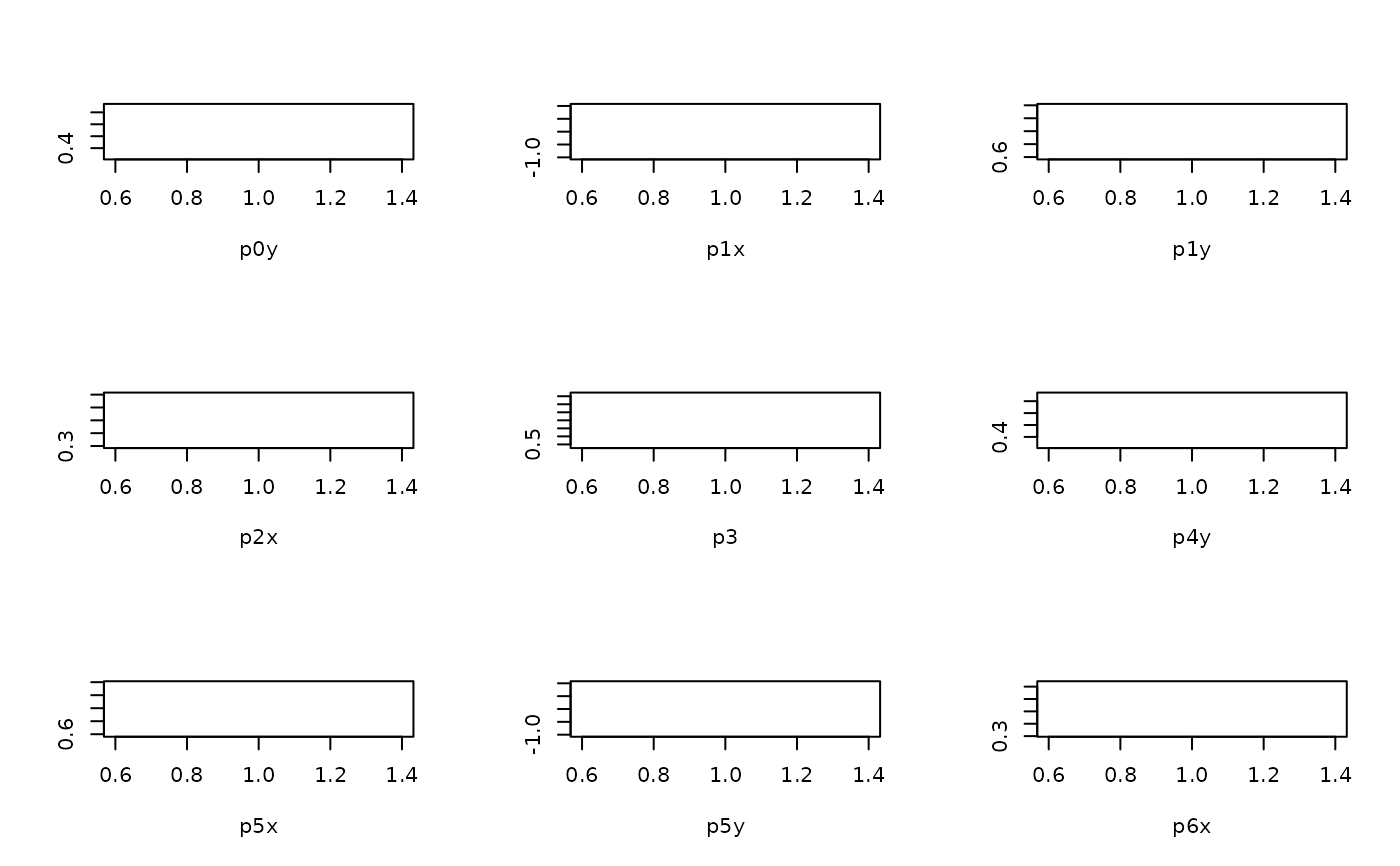
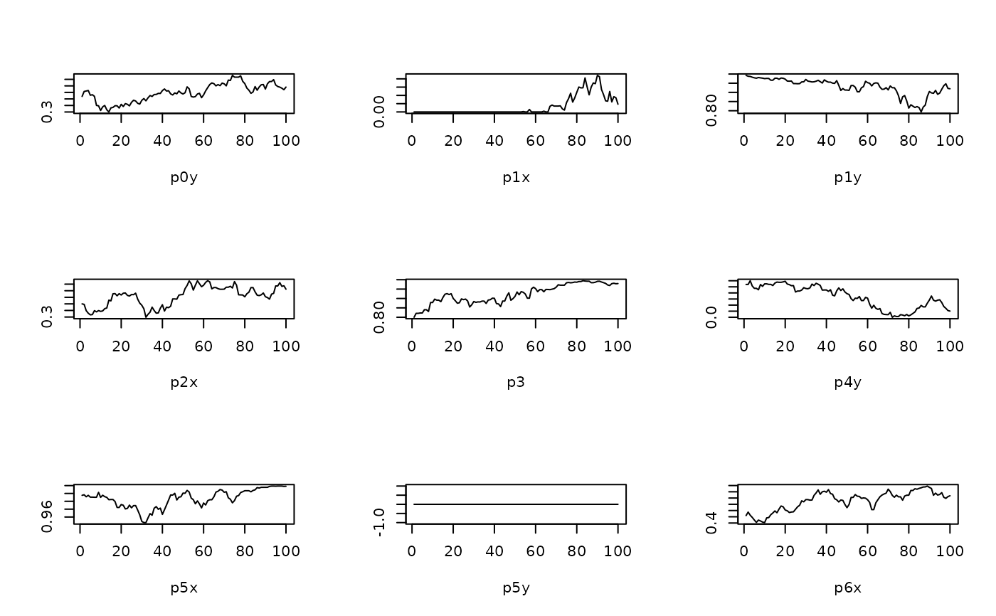
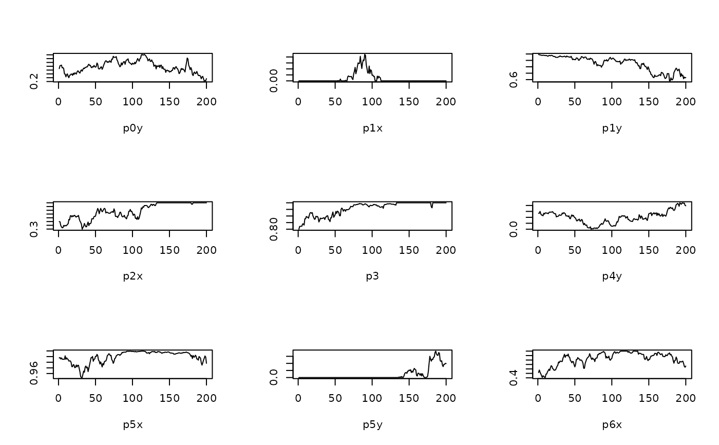
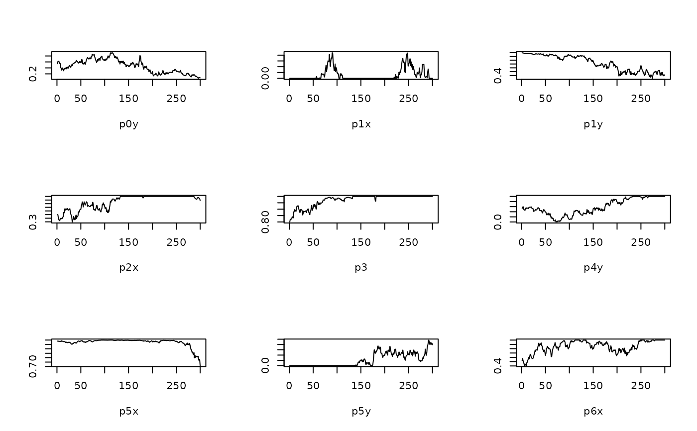
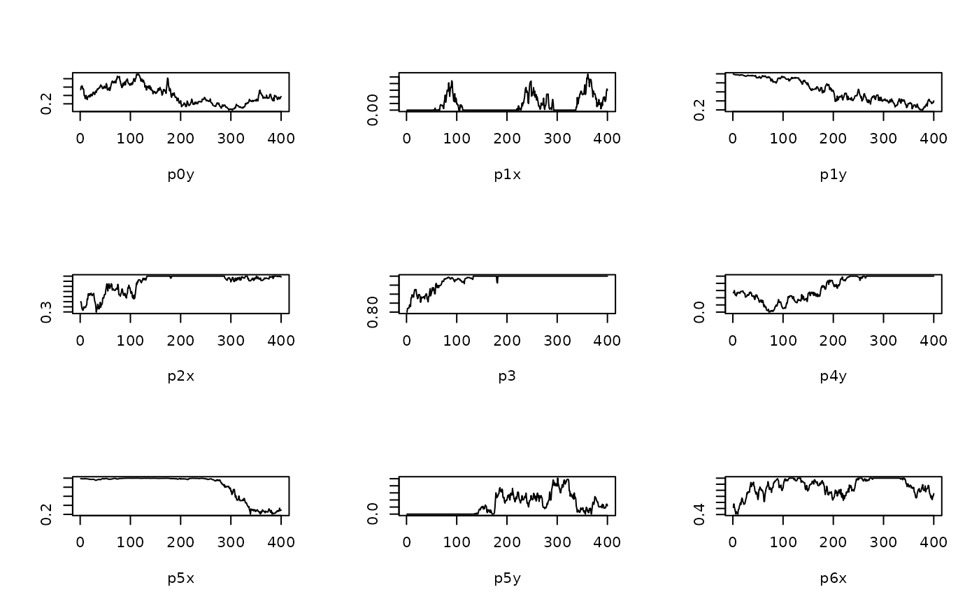
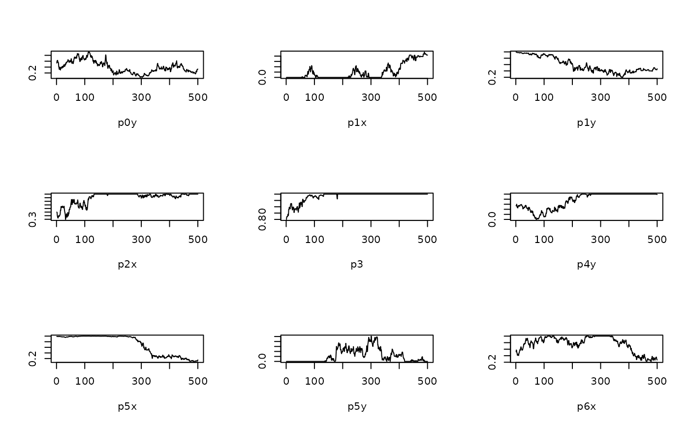
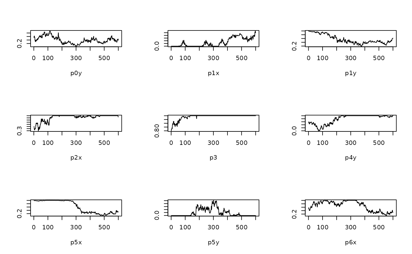
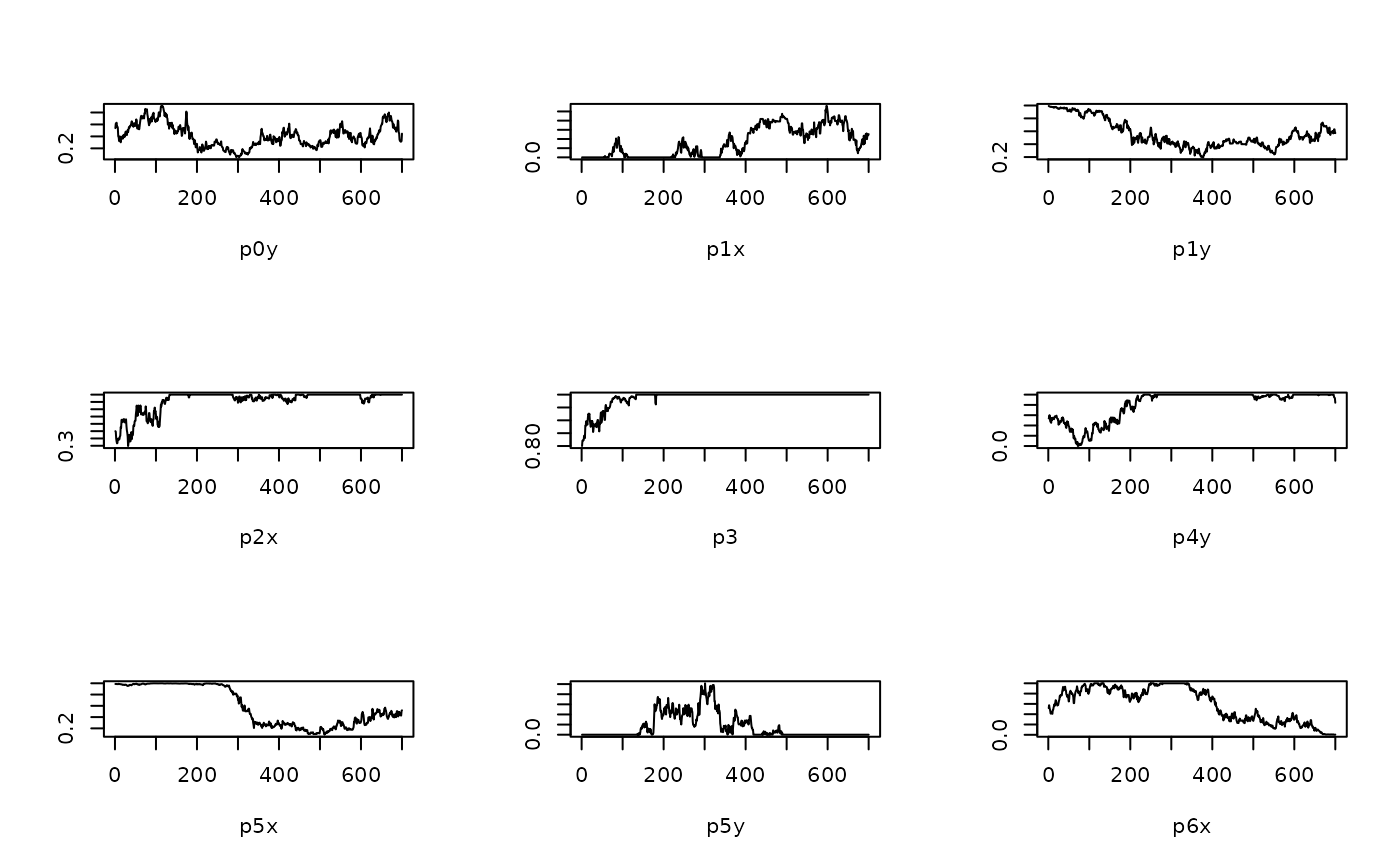
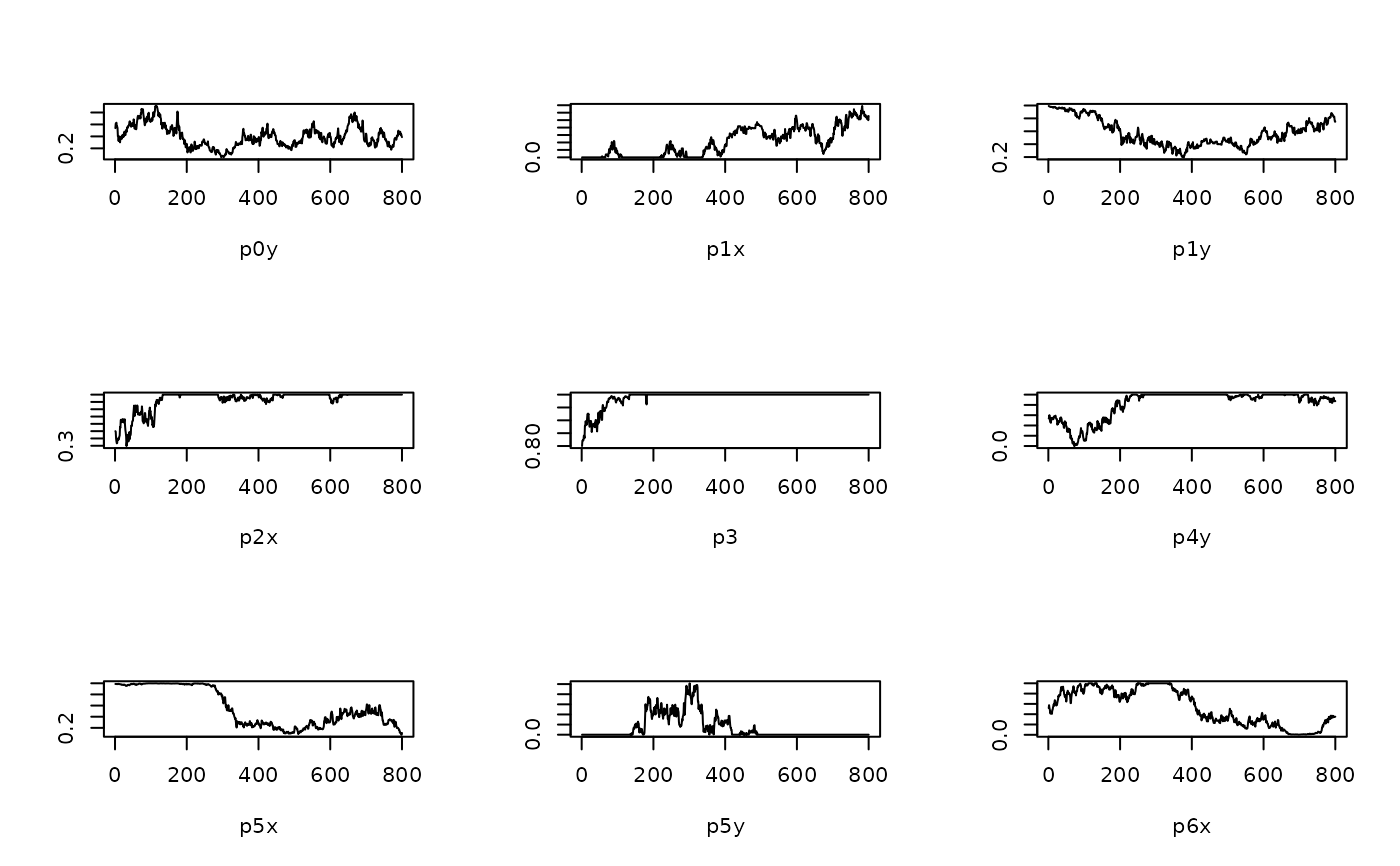
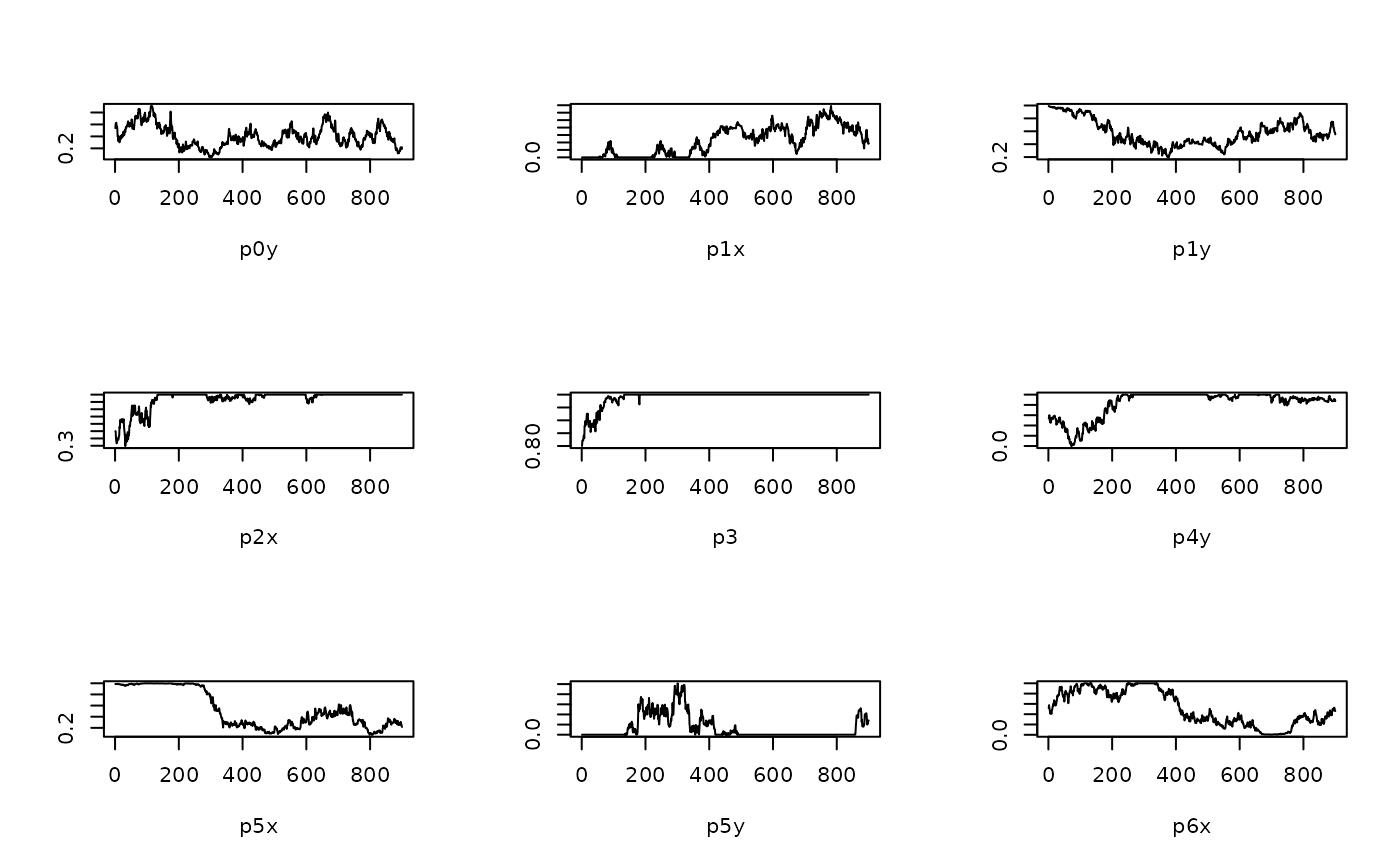
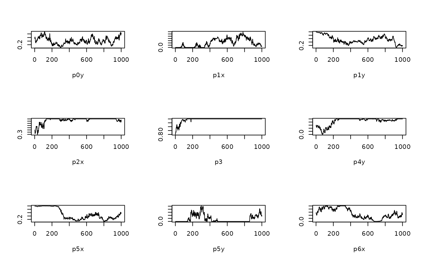
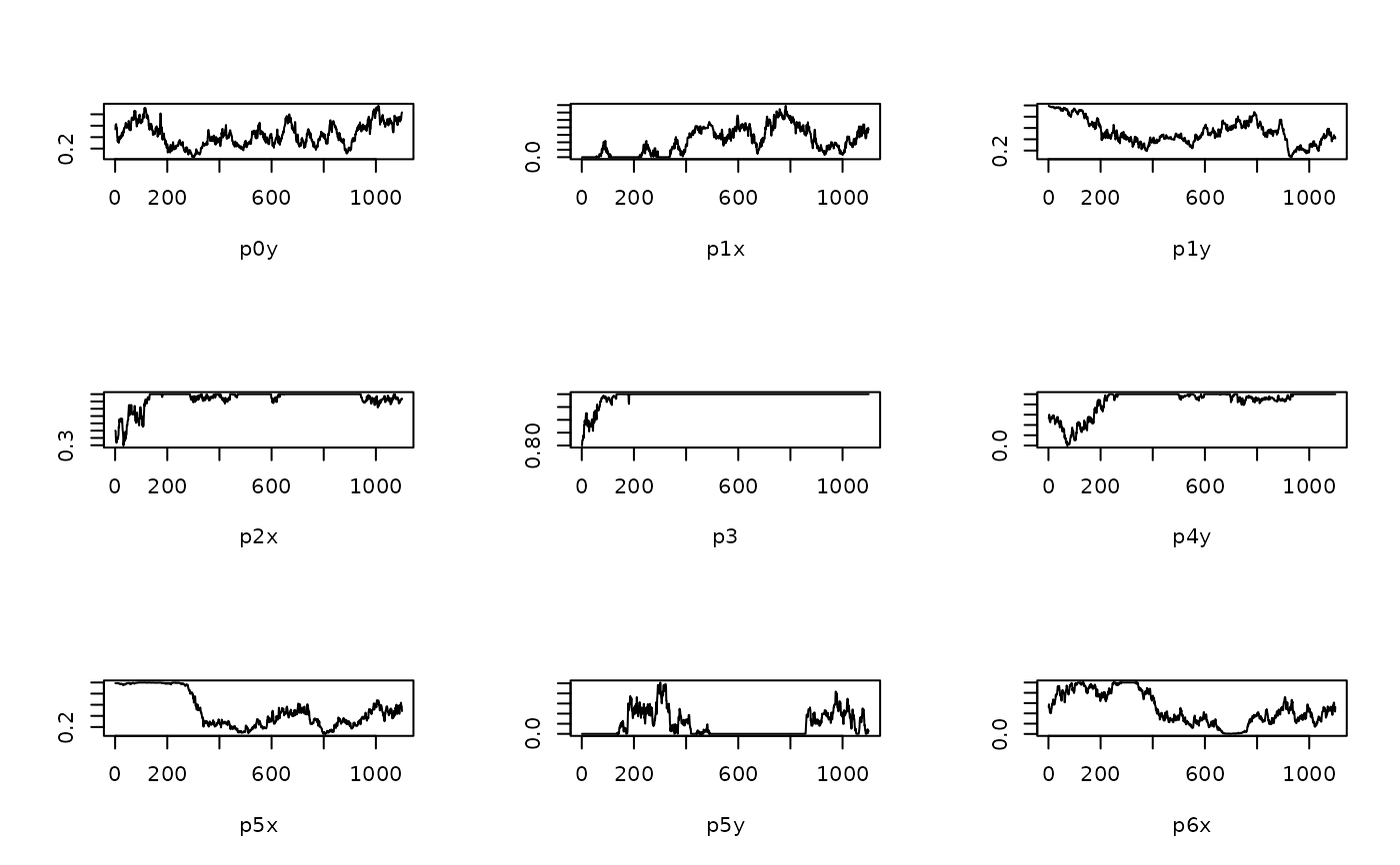
  traceplot = T
)

Arguments

N

Number of data points that the truncated Gamma distribution is to be fitted to

r

Vector of radii of length N

w

Vector of angles of length N

r_0

Vector of truncation thresholds of length N

priors

list of priors

inits

list of initial values

pmix

list of mixture components

iters

Total number of iterations

burn

Number of burn-in iterations

print.every

How many iterations between output

traceplot

Plot traceplot (TRUE/FALSE)

Value

samples Matrix of MCMC samples of Bezier control points, shape parameter, and eta

Examples

set.seed(1)
simdata             <- gen_data_exp(n = 500, theta = 0.3, tau=0.75, copula = 'l')
x                   <- simdata$x
r                   <- simdata$r
w                   <- simdata$w
data_marg_r_0       <- simdata$data_marg_r_0
samples  <- fit_mcmc_bezier( N = data_marg_r_0$N,
                         r = data_marg_r_0$r,
                         w = data_marg_r_0$w,
                         r_0 = data_marg_r_0$r_0,
                         iters = 1100, burn = 100,
                         traceplot=T, print.every = 100)
#> 1 0.54 0 0.99 0.5 0.8 0.54 0.99 0 0.52 1 // eta =  0.7801029 

#> 100 0.68 0.05 0.92 0.72 0.98 0.1 1 0 0.84 2.03 // eta =  0.876082 

#> 200 0.28 0 0.63 1 1 0.79 0.98 0.2 0.66 1.5 // eta =  1 

#> 300 0.07 0 0.42 0.89 1 1 0.71 0.4 1 2.22 // eta =  1 

#> 400 0.37 0.15 0.4 0.98 1 1 0.29 0.12 0.74 2.84 // eta =  1 

#> 500 0.33 0.42 0.47 1 1 0.99 0.15 0 0.27 3.2 // eta =  1 

#> 600 0.39 0.5 0.62 0.95 1 1 0.32 0 0.3 2.7 // eta =  1 

#> 700 0.45 0.25 0.57 1 1 0.84 0.52 0 0 2.25 // eta =  1 

#> 800 0.39 0.56 0.75 1 1 0.87 0.11 0 0.35 2.35 // eta =  1 

#> 900 0.22 0.19 0.55 1 1 0.88 0.22 0.14 0.46 2.38 // eta =  1 

#> 1000 0.82 0.04 0.2 0.9 1 1 0.58 0.18 0.49 2.63 // eta =  1 

#> 1100 0.83 0.37 0.41 0.94 1 1 0.49 0.03 0.52 2.01 // eta =  1 

median(samples[101:1100,11]) # posterior median of eta
#> [1] 1